» Download this section as PDF (opens in a new tab/window)
The Acropolis Operating System (AOS) provides the core functionality leveraged by workloads and services running on the platform. This includes, but isn’t limited to, things like storage services, upgrades, etc. Built on a foundation that doesn’t just manage resources—it optimizes them. AOS abstracts the complexity of hardware and hypervisors, using a distributed “Leader/Worker” model to ensure your workloads are always running on the best possible node without manual tuning. This translates to absolute workload mobility and proactive “hot spot” elimination through a dynamic scheduler that understands both compute and storage demands.
The figure highlights an image illustrating the conceptual nature of AOS at various layers:
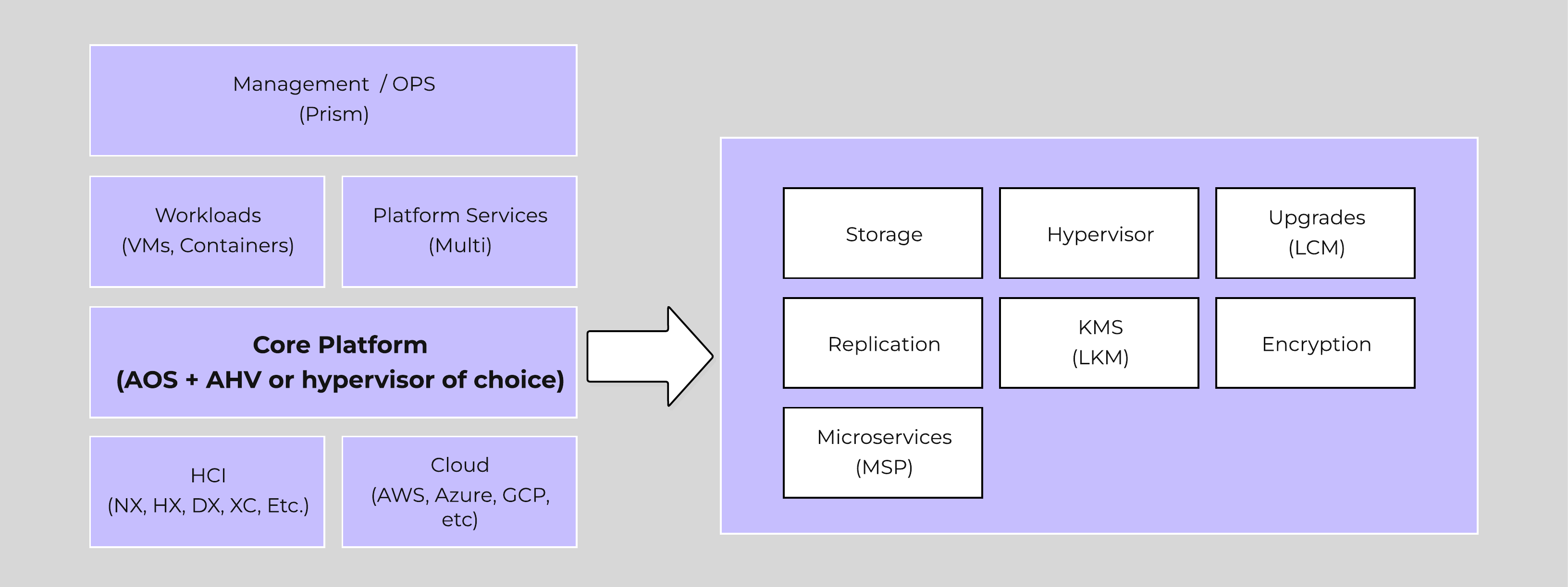 High-level AOS Architecture
Building upon the distributed nature of everything Nutanix does, we’re expanding this into the virtualization and resource management space. AOS is a back-end service that allows for workload and resource management, provisioning, and operations. Its goal is to abstract the facilitating resource (e.g., hypervisor, on-premises, cloud, etc.) from the workloads running, while providing a single “platform” to operate.
This gives workloads the ability to seamlessly move between hypervisors, cloud providers, and platforms.
AHV and ESXi are the supported hypervisors for VM management. The Volumes API and read-only operations are still supported on all.
An Acropolis Worker runs on every CVM with an elected Acropolis Leader which is responsible for task scheduling, execution, IPAM, etc. Similar to other components which have a Leader, if the Acropolis Leader fails, a new one will be elected.
The role breakdown for each can be seen below:
Here we show a conceptual view of the Acropolis Leader / Worker relationship:
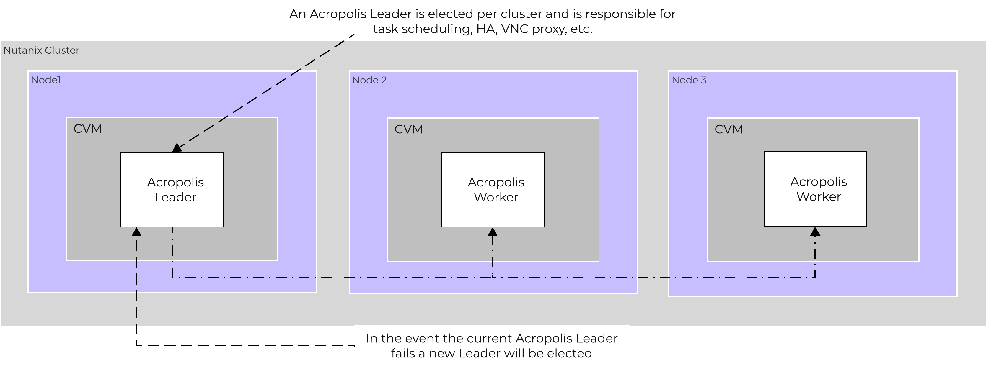 Acropolis Services
Efficient scheduling of resources is critical to ensure resources are effectively consumed. The AOS Dynamic Scheduler extends the traditional means of scheduling that relies upon compute utilization (CPU/MEM) to make placement decisions. It leverages compute, as well as storage and other statisctical data to drive VM and volume (ABS) placement decisions. This ensures that resources are effectively consumed and end-user performance is optimal.
Resource scheduling can be broken down into two key areas:
The figure shows a high-level view of the scheduler architecture:
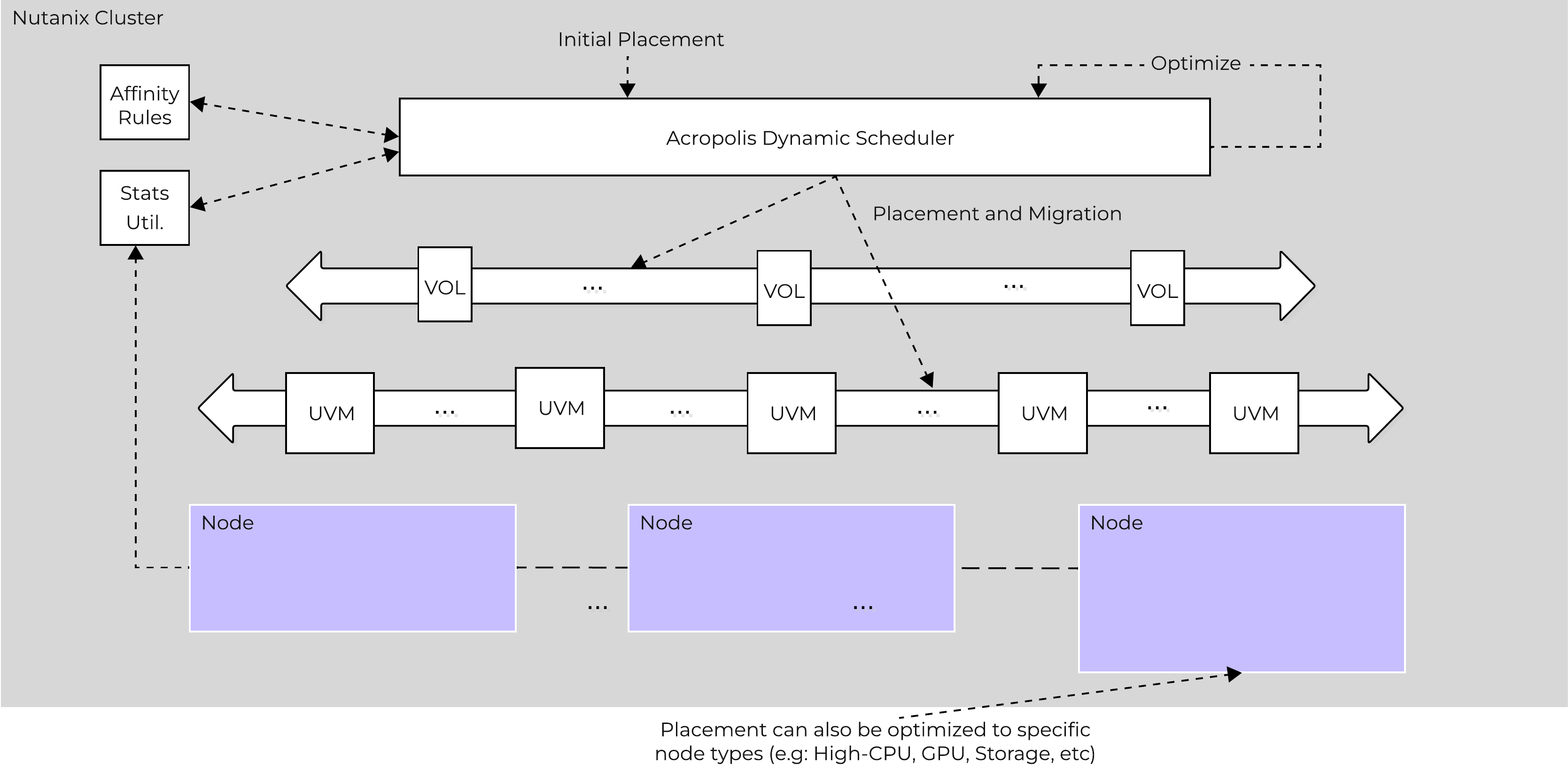 AOS Dynamic Scheduler
| The dynamic scheduler runs consistently throughout the day to optimize placement (currently every 15 minutes | Gflag: lazan_anomaly_detection_period_secs). Estimated demand is calculated using historical utilization values and fed into a smoothing algorithm. This estimated demand is what is used to determine movement, which ensures a sudden spike will not skew decisions. |
Conventional cluster schedulers were generally focused on the principle of evenly spreading workloads across available resourecs to achieve balance. NOTE: how aggressively it tries to eliminate skew is determined by the balancing configuration (e.g. manual -> none, conservative -> some, aggressive -> more).
For example, say we had 3 hosts in a cluster, each of which is utilized 50%, 5%, 5% respectively. Typical solutions would try to re-balance workloads to get each hosts utilization ~20%. But why?
What we're really trying to do is eliminate / negate any contention for resources, not eliminate skew. Unless there is contention for resources there is no positive gain from "balancing" workloads. In fact by forcing unnecessary movement it can cause additional requisite work (e.g. memory transfer, cache re-localization, etc.), all of which consumes resources.
The AOS Dynamic Scheduler focuses more on alleviating hot spots. It will only invoke workload movement if there is expected contention for resources, not because of skew. NOTE: DSF works in a different way and works to ensure uniform distribution of data throughout the cluster to eliminate hot spots and speed up rebuilds. To learn more of DSF, check out the 'disk balancing' section.
At power-on ADS will balance VM initial placement throughout the cluster.
Placement decisions are based upon the following items:
| We monitor each individual node’s compute utilization. In the event where a node’s expected CPU allocation breaches its threshold (currently 85% of host CPU | Gflag: lazan_host_cpu_usage_threshold_fraction) we will migrate VMs off those host(s) to re-balance the workload. A key thing to mention here is a migration will only be performed when there is contention. If there is skew in utilization between nodes (e.g. 3 nodes at 10% and 1 at 50%) we will not perform a migration as there is no benefit from doing so until there is contention for resources. |
| Being a hyperconverged platform we manage both compute and storage resources. The scheduler will monitor each node’s Stargate process utilization. In the event where certain Stargate(s) breach their allocation threshold (currently 85% of CPU allocated to Stargate | Gflag: lazan_stargate_cpu_usage_threshold_pct) , we will migrate resources across hosts to eliminate any hot spots. Both VMs and ABS Volumes can be migrated to eliminate any hot Stargates. |
The scheduler will make its best effort to optimize workload placement based upon the prior items. The system places a penalty on movement to ensure not too many migrations are taking place. This is a key item as we want to make sure the movement doesn’t have any negative impacts on the workload.
After a migration the system will judge its “effectiveness” and see what the actual benefit is. This learning model can self-optimize to ensure there is a valid basis for any migration decision.
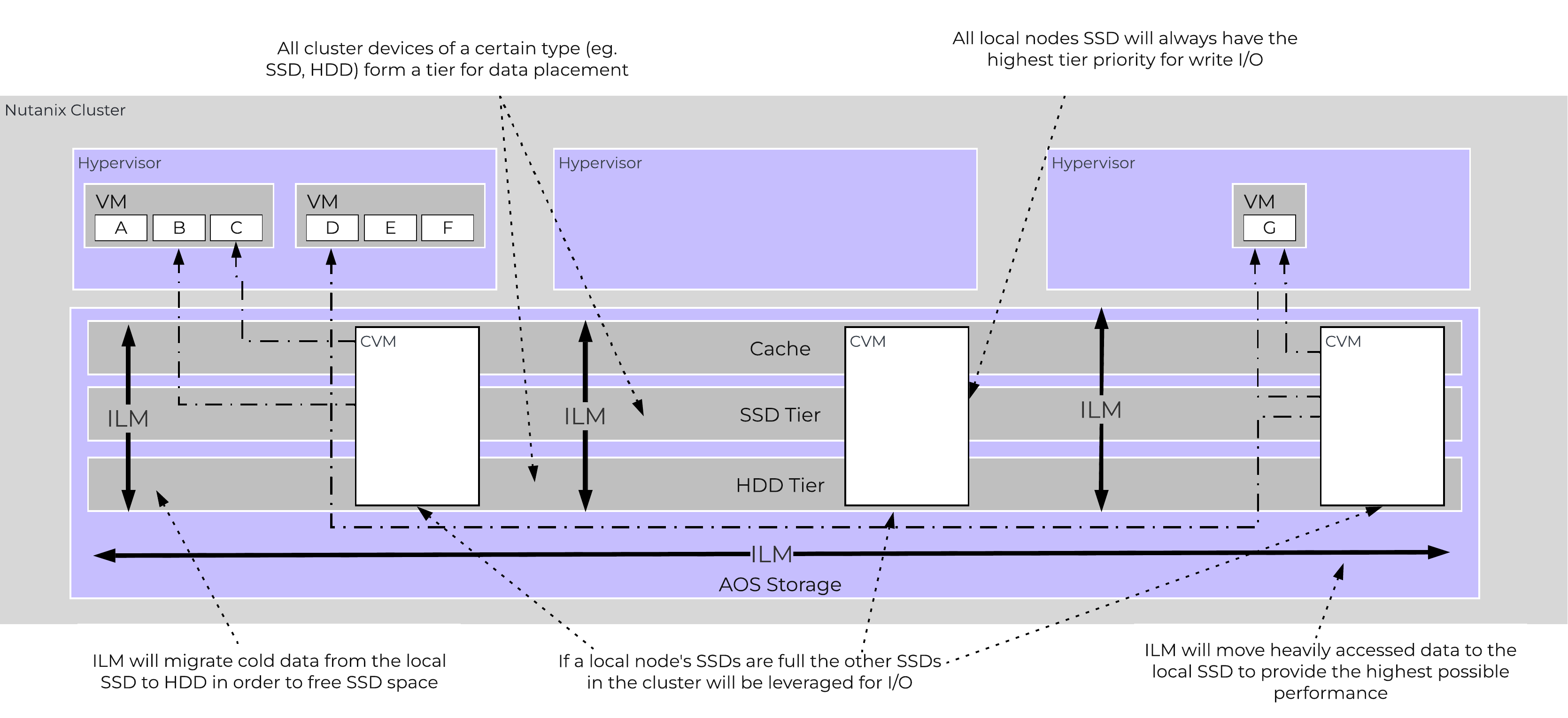
The Disk Balancing section below talks about how storage capacity was pooled among all nodes in a Nutanix cluster and that ILM would be used to keep hot data local. A similar concept applies to disk tiering, in which the cluster’s SSD and HDD tiers are cluster-wide and AOS ILM is responsible for triggering data movement events. A local node’s SSD tier is always the highest priority tier for all I/O generated by VMs running on that node, however all of the cluster’s SSD resources are made available to all nodes within the cluster. The SSD tier will always offer the highest performance and is a very important thing to manage for hybrid arrays.
The tier prioritization can be classified at a high-level by the following:
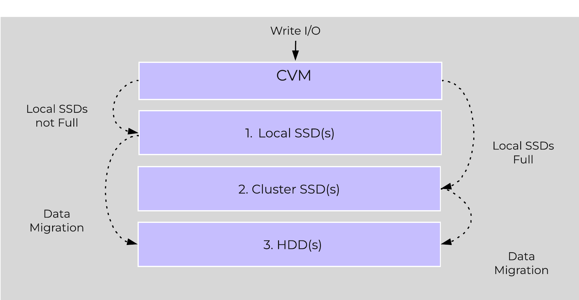 AOS Tier Prioritization
Specific types of resources (e.g. SSD, HDD, etc.) are pooled together and form a cluster wide storage tier. This means that any node within the cluster can leverage the full tier capacity, regardless if it is local or not.
The following figure shows a high level example of what this pooled tiering looks like:
 AOS Cluster-wide Tiering
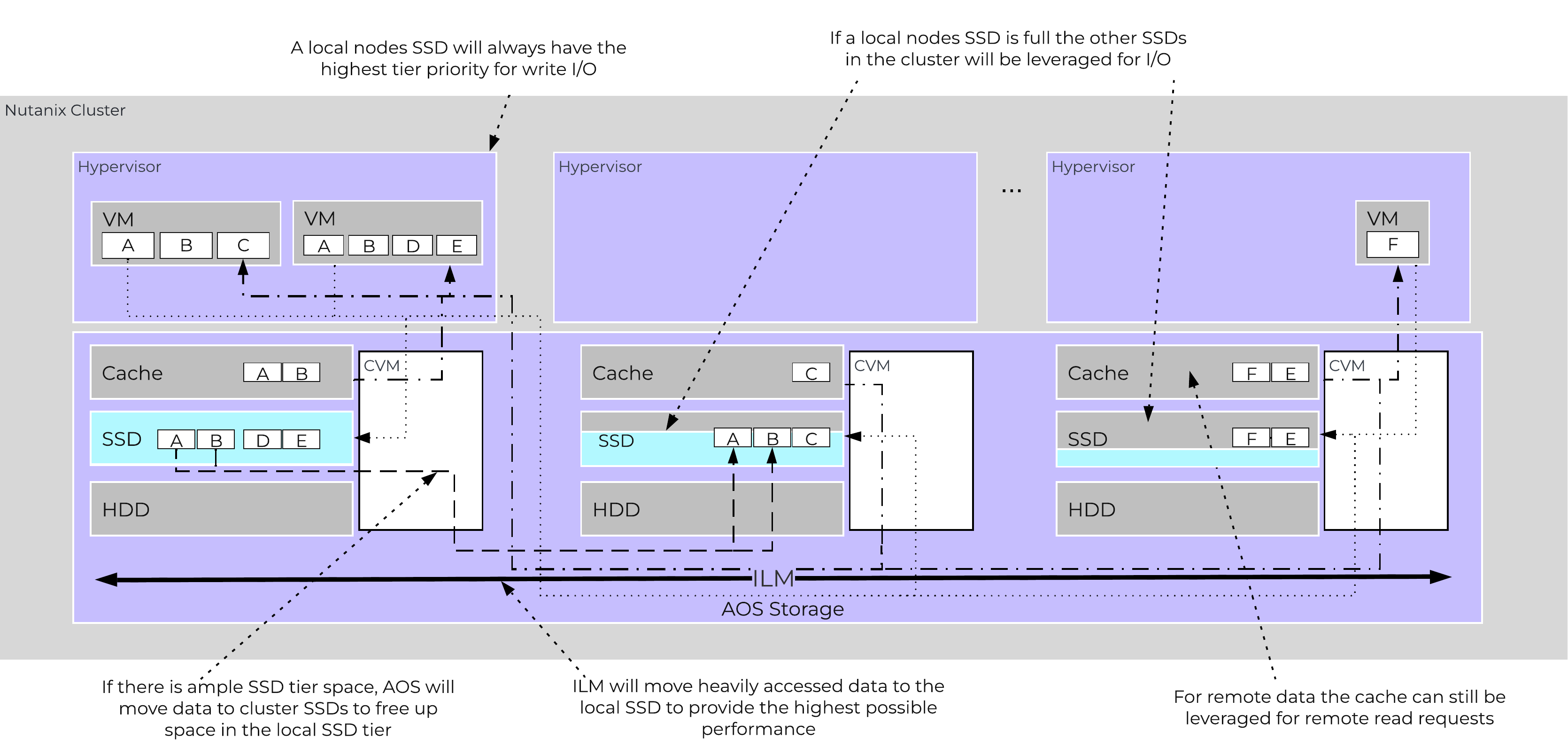
A common question is what happens when a local node’s SSD becomes full? As mentioned in the Disk Balancing section, a key concept is trying to keep uniform utilization of devices within disk tiers. In the case where a local node’s SSD utilization is high, disk balancing will kick in to move the coldest data on the local SSDs to the other SSDs throughout the cluster. This will free up space on the local SSD to allow the local node to write to SSD locally instead of going over the network. A key point to mention is that all CVMs and SSDs are used for this remote I/O to eliminate any potential bottlenecks and remediate some of the hit by performing I/O over the network.
 AOS Cluster-wide Tier Balancing
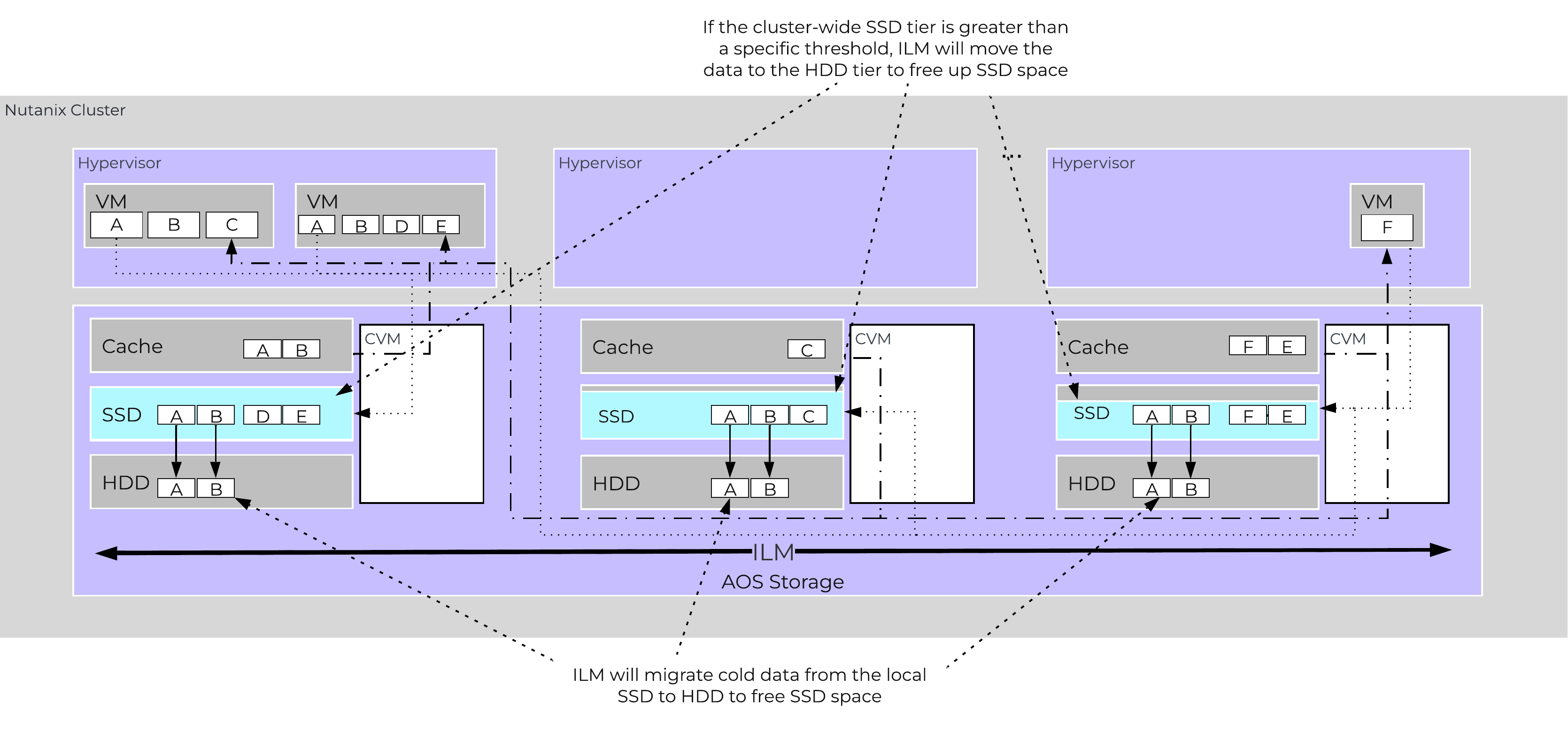
The other case is when the overall tier utilization breaches a specific threshold [curator_tier_usage_ilm_threshold_percent (Default=75)] where AOS ILM will kick in and as part of a Curator job will down-migrate data from the SSD tier to the HDD tier. This will bring utilization within the threshold mentioned above or free up space by the following amount [curator_tier_free_up_percent_by_ilm (Default=15)], whichever is greater. The data for down-migration is chosen using last access time. In the case where the SSD tier utilization is 95%, 20% of the data in the SSD tier will be moved to the HDD tier (95% –> 75%).
However, if the utilization was 80%, only 15% of the data would be moved to the HDD tier using the minimum tier free up amount.
 AOS Tier ILM
AOS ILM will constantly monitor the I/O patterns and (down/up) migrate data as necessary as well as bring the hottest data local regardless of tier. The logic for up-migration (or horizontal) follows the same as that defined for egroup locality: “3 touches for random or 10 touches for sequential within a 10 minute window where multiple reads every 10 second sampling count as a single touch”.
For a visual explanation, you can watch the following video: LINK
AOS is designed to be a very dynamic platform which can react to various workloads as well as allow heterogeneous node types: compute heavy (3155, 9151, etc.) and storage heavy (8150, etc.) to be mixed in a single cluster. Ensuring uniform distribution of data is an important item when mixing nodes with larger storage capacities. AOS has a native feature, called disk balancing, which is used to ensure uniform distribution of data throughout the cluster. Disk balancing works on a node’s utilization of its local storage capacity and is integrated with AOS ILM. Its goal is to keep utilization uniform among nodes once the utilization has breached a certain threshold.
NOTE: Disk balancing jobs are handled by Curator which has different priority queues for primary I/O (UVM I/O) and background I/O (e.g. disk balancing). This is done to ensure disk balancing or any other background activity doesn’t impact front-end latency / performance. In this cases the job’s tasks will be given to Chronos who will throttle / control the execution of the tasks. Also, movement is done within the same tier for disk balancing. For example, if data is skewed in the HDD tier, it can be moved amongst nodes in the same tier.
The following figure shows an example of a mixed cluster (3060 + 8150) in an “unbalanced” state:
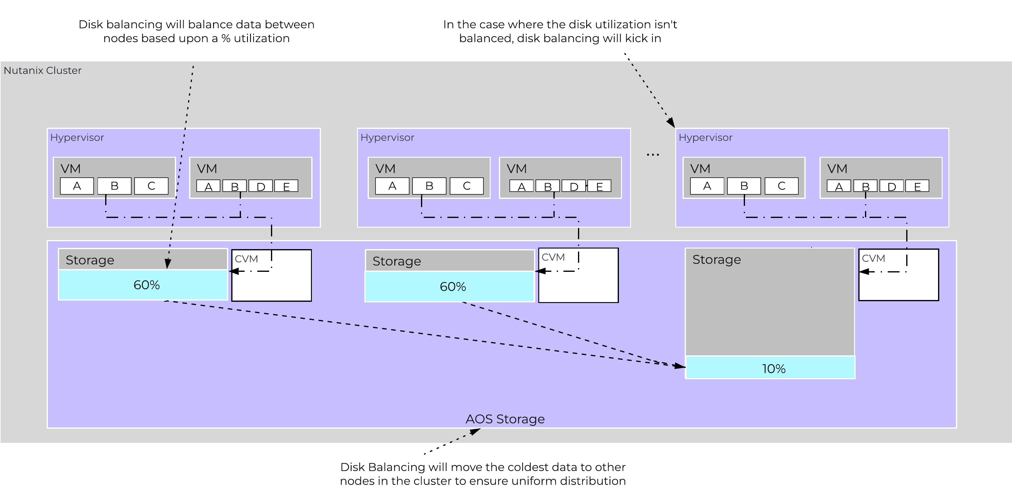 Disk Balancing - Unbalanced State
Disk balancing leverages the AOS Curator framework and is run as a scheduled process as well as when a threshold has been breached (e.g., local node capacity utilization > n %). In the case where the data is not balanced, Curator will determine which data needs to be moved and will distribute the tasks to nodes in the cluster. In the case where the node types are homogeneous (e.g., 3060), utilization should be fairly uniform. However, if there are certain VMs running on a node which are writing much more data than others, this can result in a skew in the per node capacity utilization. In this case, disk balancing would run and move the coldest data on that node to other nodes in the cluster. In the case where the node types are heterogeneous (e.g., 3060 + 8150/55/70), or where a node may be used in a “storage only” mode (not running any VMs), there will likely be a requirement to move data.
The following figure shows an example the mixed cluster after disk balancing has been run in a “balanced” state:
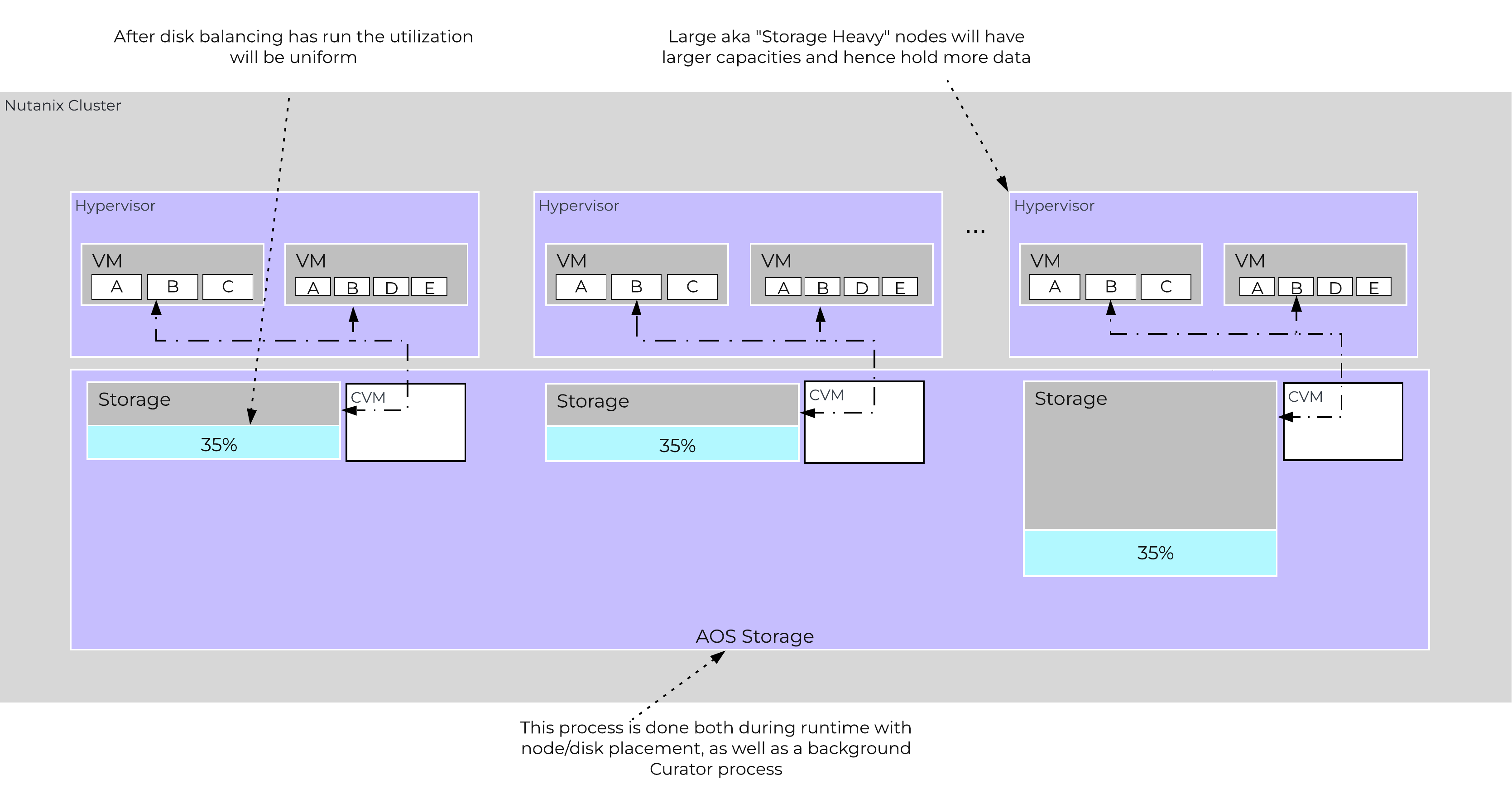 Disk Balancing - Balanced State
In some scenarios, customers might run some nodes in a “storage-only” state where only the CVM will run on the node whose primary purpose is bulk storage capacity. In this case, the full node’s memory can be added to the CVM to provide a much larger read cache.
The following figure shows an example of how a storage only node would look in a mixed cluster with disk balancing moving data to it from the active VM nodes:
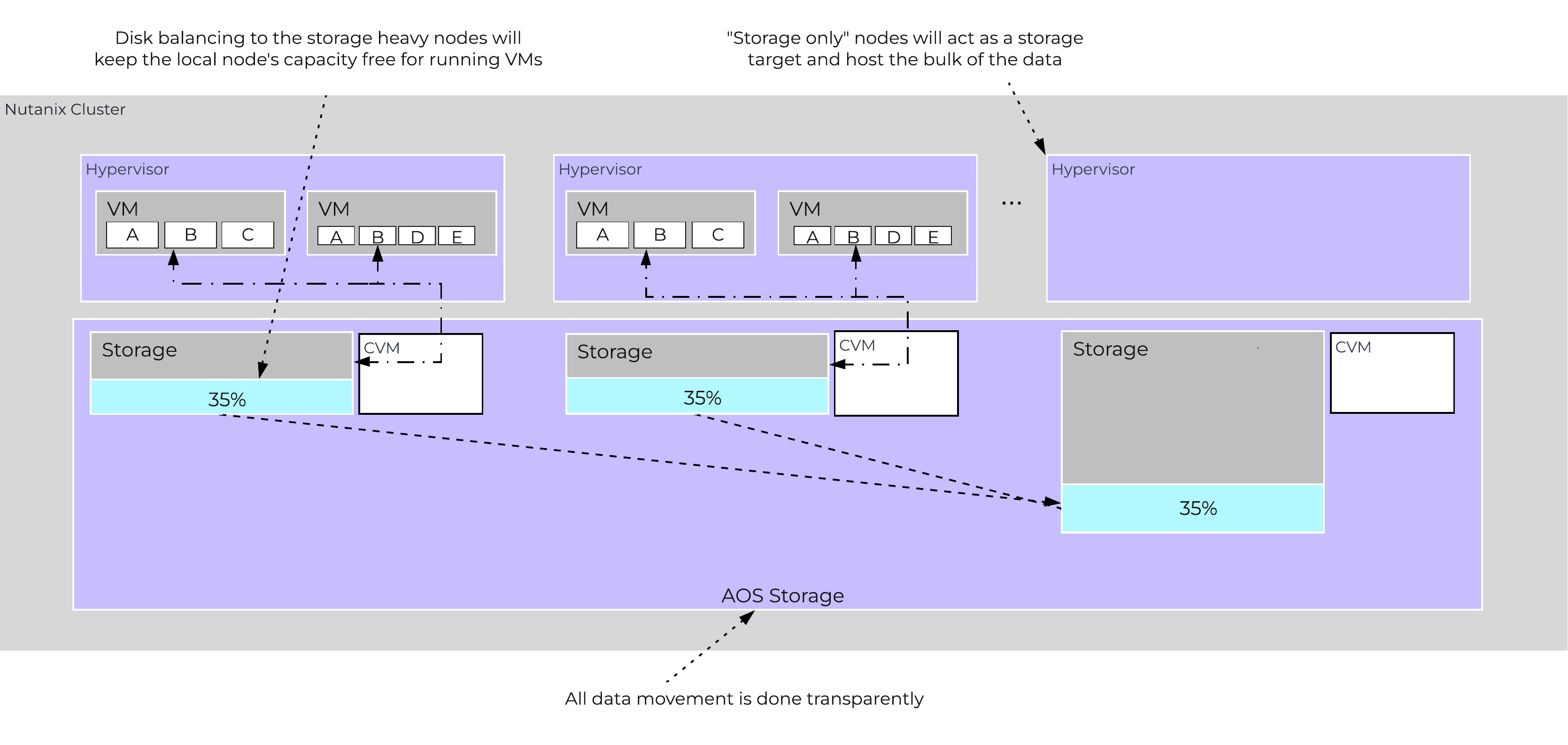 Disk Balancing - Storage Only Node
For a visual explanation, you can watch the following video: LINK
AOS provides native support for offloaded snapshots and clones which can be leveraged via VAAI, ODX, ncli, REST, Prism, etc. Both the snapshots and clones leverage the redirect-on-write algorithm which is the most effective and efficient. As explained in the Data Structure section above, a virtual machine consists of files (vmdk/vhdx) which are vDisks on the Nutanix platform.
A vDisk is composed of extents which are logically contiguous chunks of data, which are stored within extent groups which are physically contiguous data stored as files on the storage devices. When a snapshot or clone is taken, the base vDisk is marked immutable and another vDisk is created as read/write. At this point, both vDisks have the same block map, which is a metadata mapping of the vDisk to its corresponding extents. Contrary to traditional approaches which require traversal of the snapshot chain (which can add read latency), each vDisk has its own block map. This eliminates any of the overhead normally seen by large snapshot chain depths and allows you to take continuous snapshots without any performance impact.
The following figure shows an example of how this works when a snapshot is taken (source: NTAP):
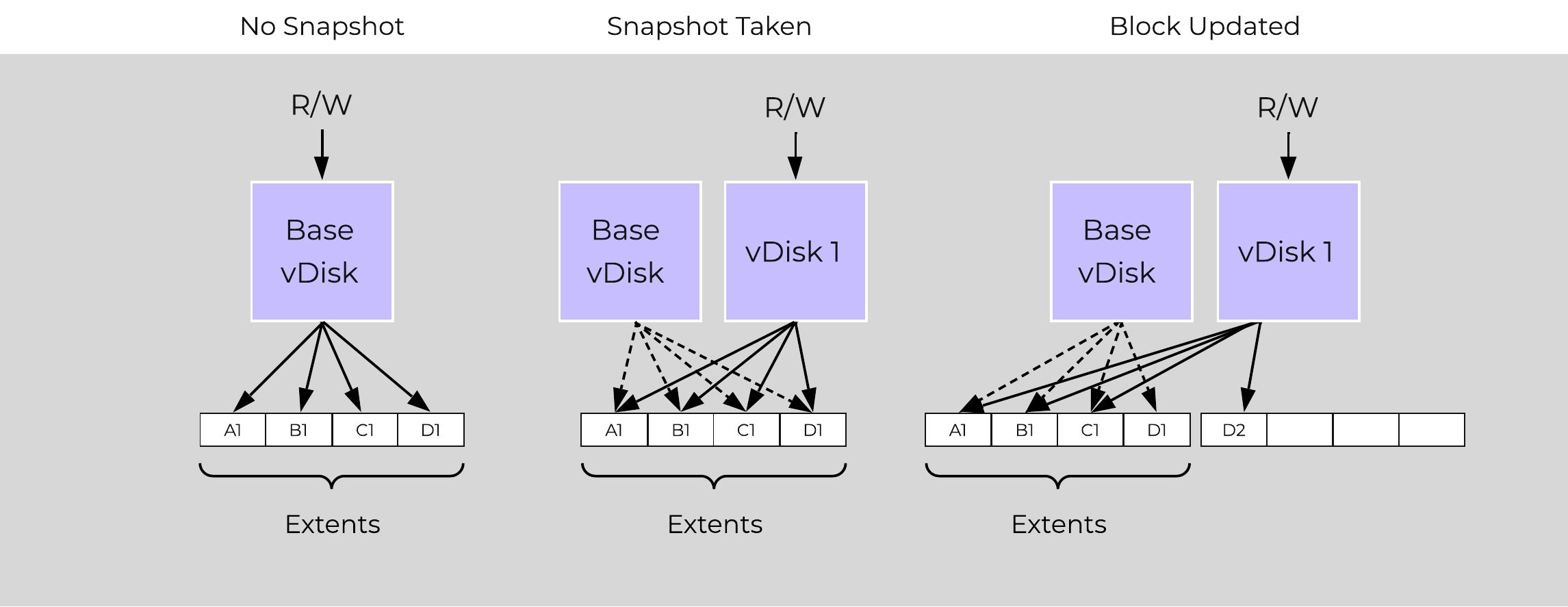 Example Snapshot Block Map
The same method applies when a snapshot or clone of a previously snapped or cloned vDisk is performed:
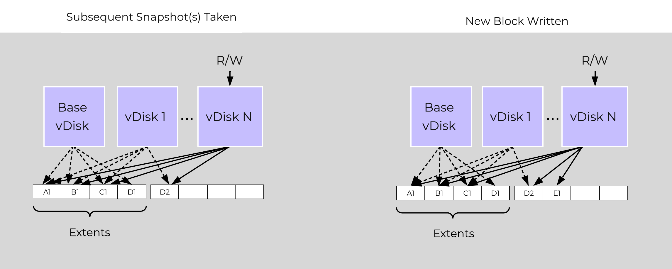 Multi-snap Block Map and New Write
The same methods are used for both snapshots and/or clones of a VM or vDisk(s). When a VM or vDisk is cloned, the current block map is locked and the clones are created. These updates are metadata only, so no I/O actually takes place. The same method applies for clones of clones; essentially the previously cloned VM acts as the “Base vDisk” and upon cloning, that block map is locked and two “clones” are created: one for the VM being cloned and another for the new clone. There is no imposed limit on the maximum number of clones.
They both inherit the prior block map and any new writes/updates would take place on their individual block maps.
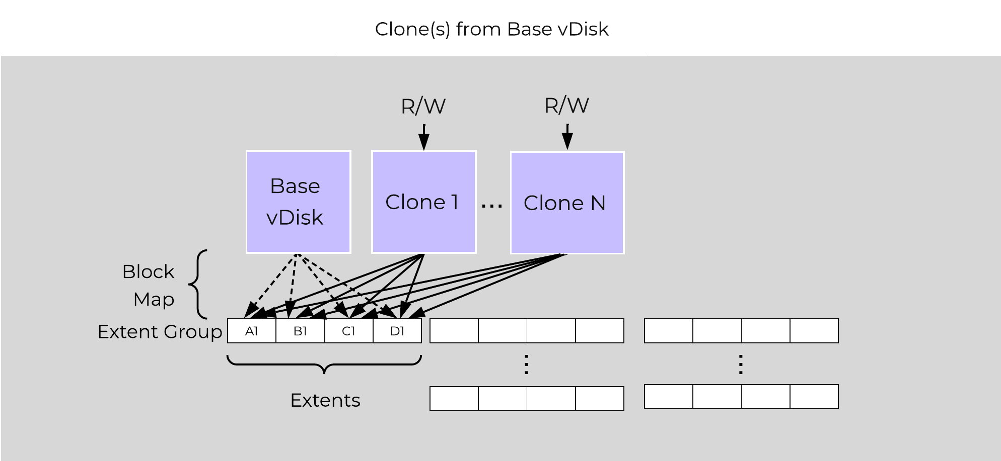 Multi-Clone Block Maps
As mentioned previously, each VM/vDisk has its own individual block map. So in the above example, all of the clones from the base VM would now own their block map and any write/update would occur there.
In the event of an overwrite the data will go to a new extent / extent group. For example, if data exists at offset o1 in extent e1 that was being overwritten, Stargate would create a new extent e2 and track that the new data was written in extent e2 at offset o2. The Vblock map tracks this down to the byte level.
The following figure shows an example of what this looks like:
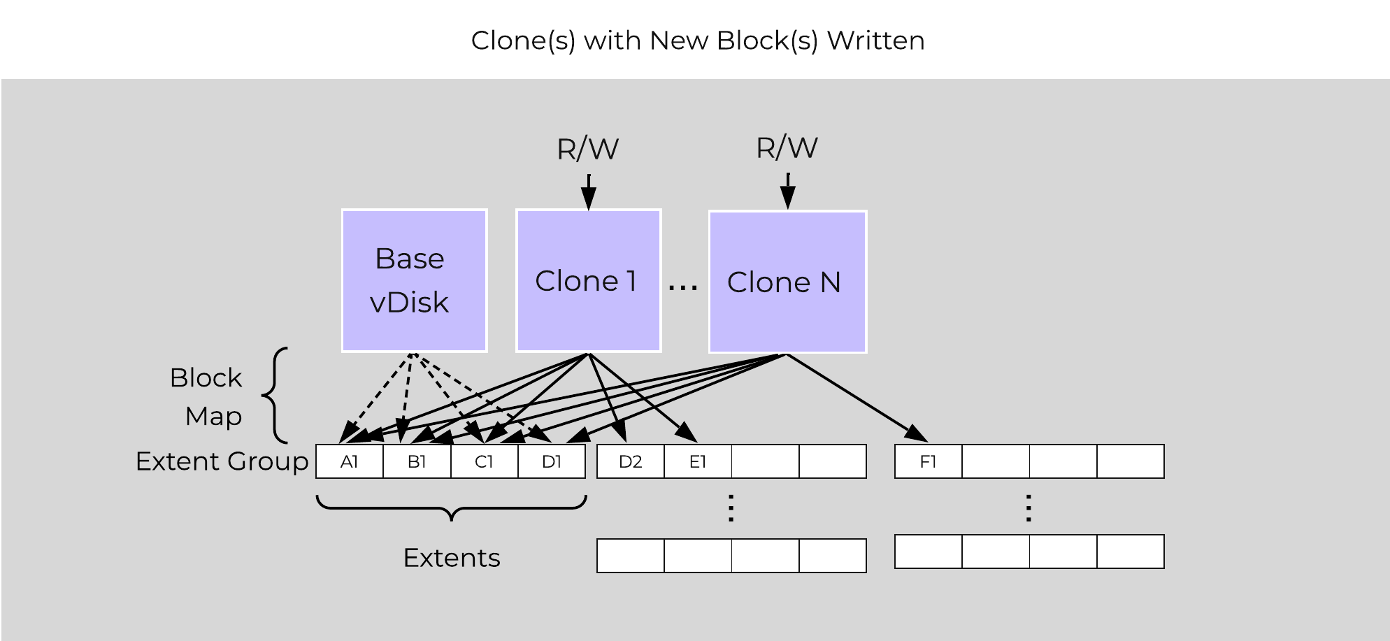 Clone Block Maps - New Write
Any subsequent clones or snapshots of a VM/vDisk would cause the original block map to be locked and would create a new one for R/W access.
The Nutanix platform does not leverage any backplane for inter-node communication and only relies on a standard 10GbE network. All storage I/O for VMs running on a Nutanix node is handled by the hypervisor on a dedicated private network. The I/O request will be handled by the hypervisor, which will then forward the request to the private IP on the local CVM. The CVM will then perform the remote replication with other Nutanix nodes using its external IP over the public 10GbE network. For all read requests, these will be served completely locally in most cases and never touch the 10GbE network. This means that the only traffic touching the public 10GbE network will be AOS remote replication traffic and VM network I/O. There will, however, be cases where the CVM will forward requests to other CVMs in the cluster in the case of a CVM being down or data being remote. Also, cluster-wide tasks, such as disk balancing, will temporarily generate I/O on the 10GbE network.
The following figure shows an example of how the VM’s I/O path interacts with the private and public 10GbE network:
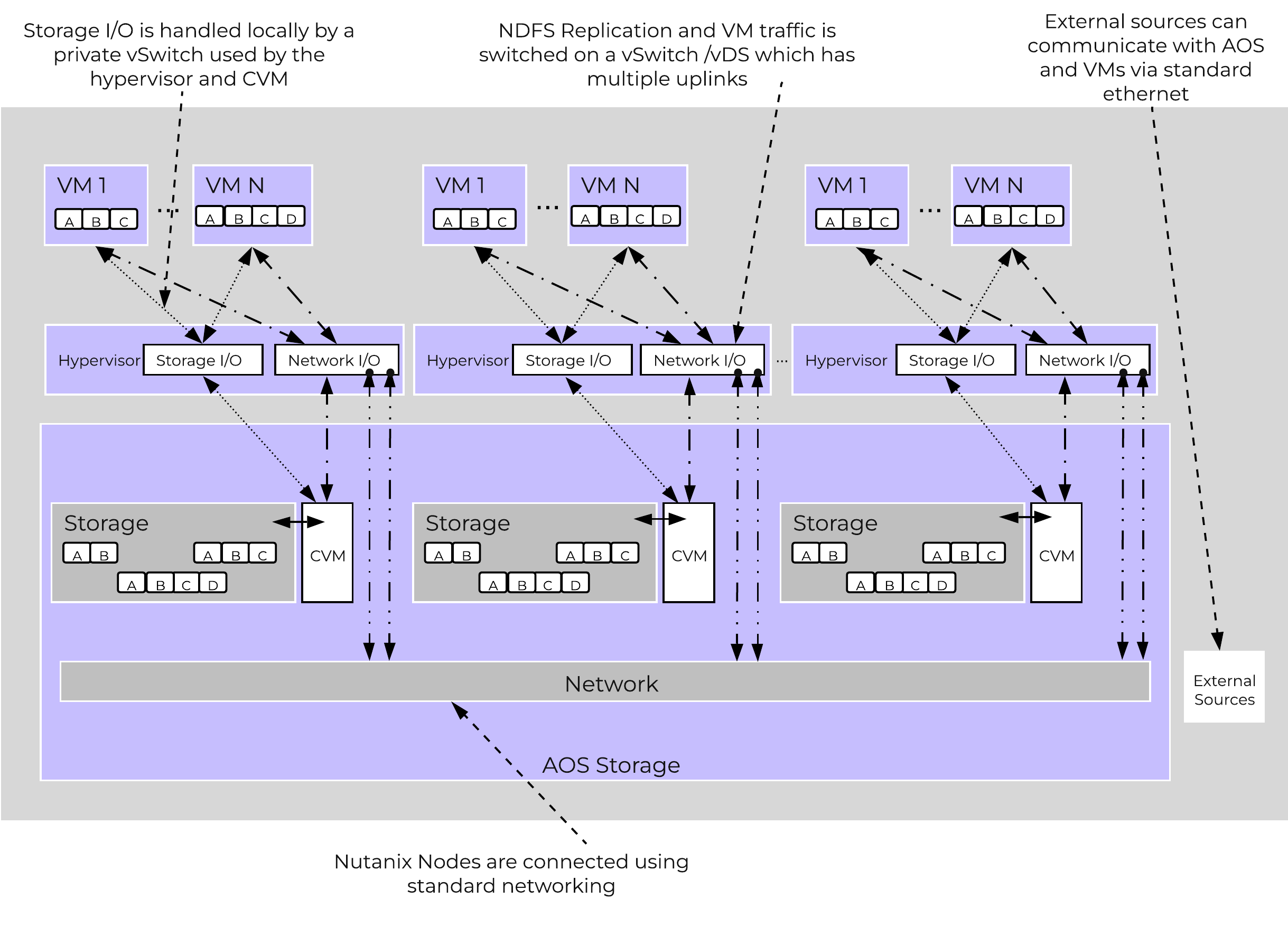 AOS Networking
Being a converged (compute+storage) platform, I/O and data locality are critical to cluster and VM performance with Nutanix. As explained above in the I/O path, all read/write IOs are served by the local Controller VM (CVM) which is on each hypervisor adjacent to normal VMs. A VM’s data is served locally from the CVM and sits on local disks under the CVM’s control. When a VM is moved from one hypervisor node to another (or during a HA event), the newly migrated VM’s data will be served by the now local CVM. When reading old data (stored on the now remote node/CVM), the I/O will be forwarded by the local CVM to the remote CVM. All write I/Os will occur locally right away. AOS will detect the I/Os are occurring from a different node and will migrate the data locally in the background, allowing for all read I/Os to now be served locally. The data will only be migrated on a read as to not flood the network.
Data locality occurs in two main flavors:
The following figure shows an example of how data will “follow” the VM as it moves between hypervisor nodes:
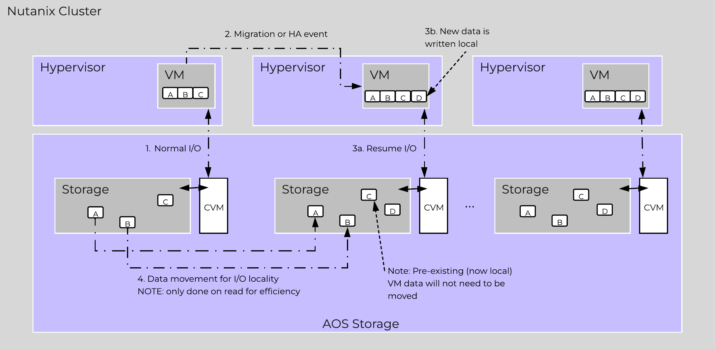 Data Locality
Cache locality occurs in real time and will be determined based upon vDisk ownership. When a vDisk / VM moves from one node to another the "ownership" of those vDisk(s) will transfer to the now local CVM. Once the ownership has transferred the data can be cached locally in the Unified Cache. In the interim the cache will be wherever the ownership is held (the now remote host). The previously hosting Stargate will relinquish the vDisk token when it sees remote I/Os for 300+ seconds at which it will then be taken by the local Stargate. Cache coherence is enforced as ownership is required to cache the vDisk data.
Egroup locality is a sampled operation and an extent group will be migrated when the following occurs: "3 touches for random or 10 touches for sequential within a 10 minute window where multiple reads every 10 second sampling count as a single touch".
AOS Storage has a feature called ‘Shadow Clones’, which allows for distributed caching of particular vDisks or VM data which is in a ‘multi-reader’ scenario. A great example of this is during a VDI deployment many ‘linked clones’ will be forwarding read requests to a central master or ‘Base VM’. In the case of Omnissa Horizon (formerly Horizon View), this is called the replica disk and is read by all linked clones, and in XenDesktop, this is called the MCS Master VM. This will also work in any scenario which may be a multi-reader scenario (e.g., deployment servers, repositories, etc.). Data or I/O locality is critical for the highest possible VM performance and a key struct of AOS.
With Shadow Clones, AOS will monitor vDisk access trends similar to what it does for data locality. However, in the case there are requests occurring from more than two remote CVMs (as well as the local CVM), and all of the requests are read I/O, the vDisk will be marked as immutable. Once the disk has been marked as immutable, the vDisk can then be cached locally by each CVM making read requests to it (aka Shadow Clones of the base vDisk). This will allow VMs on each node to read the Base VM’s vDisk locally. In the case of VDI, this means the replica disk can be cached by each node and all read requests for the base will be served locally. NOTE: The data will only be migrated on a read as to not flood the network and allow for efficient cache utilization. In the case where the Base VM is modified, the Shadow Clones will be dropped and the process will start over. Shadow clones are enabled by default and can be enabled/disabled using the following NCLI command: ncli cluster edit-params enable-shadow-clones=<true/false>.
The following figure shows an example of how Shadow Clones work and allow for distributed caching:
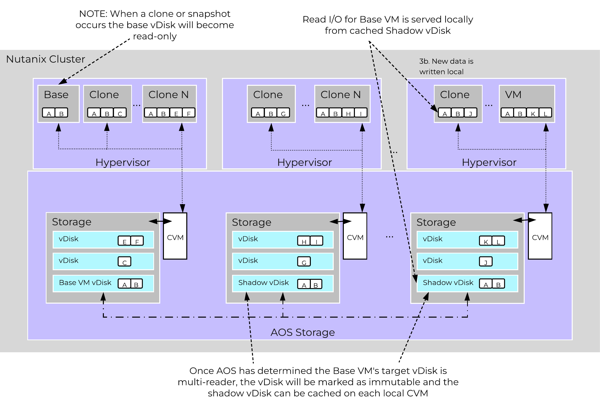 Shadow Clones
The Nutanix platform monitors storage at multiple layers throughout the stack, ranging from the VM/Guest OS all the way down to the physical disk devices. Knowing the various tiers and how these relate is important whenever monitoring the solution and allows you to get full visibility of how the ops relate. The following figure shows the various layers of where operations are monitored and the relative granularity which are explained below:
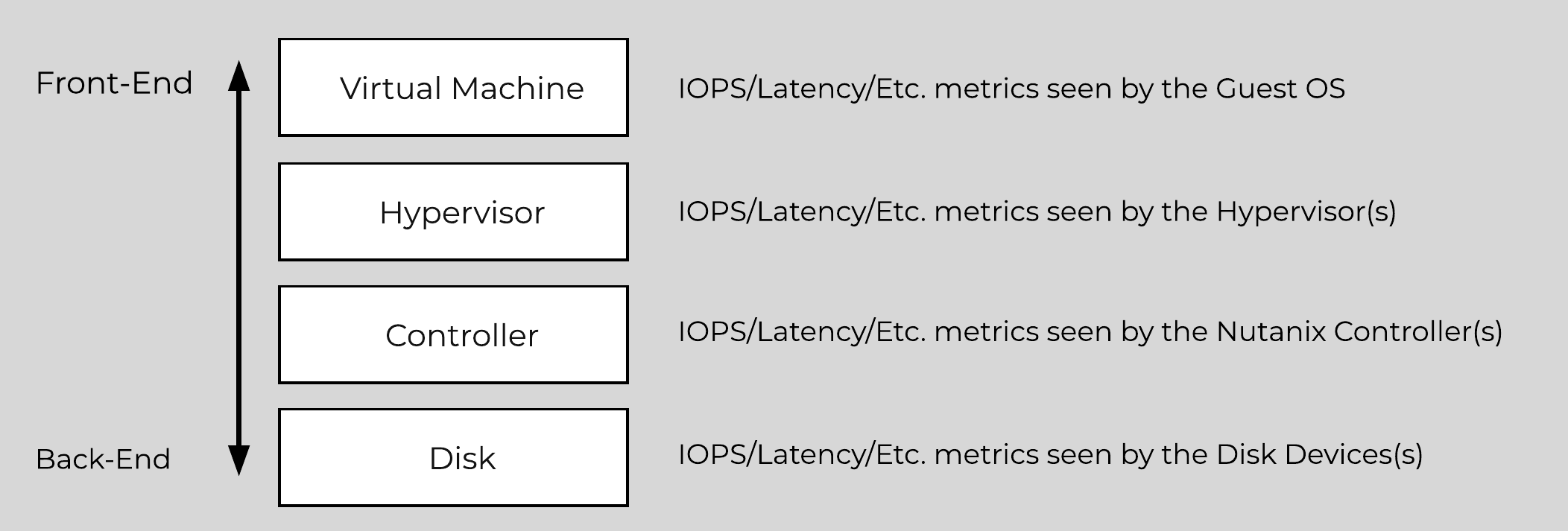 Storage Layers
Metrics and time series data is stored locally for 90 days in Prism Element. For Prism Central and Insights, data can be stored indefinitely (assuming capacity is available).
©2025 Nutanix, Inc. All rights reserved. Nutanix, the Nutanix logo and all Nutanix product and service names mentioned are registered trademarks or trademarks of Nutanix, Inc. in the United States and other countries. All other brand names mentioned are for identification purposes only and may be the trademarks of their respective holder(s).